Debugging
A collection of issues I've consistently encountered over time, and the fixes for them.
Exit code 137
Usually indicates some sort of Out-Of-Memory (OOM) error. Was the case on my HPC job when my np.load was allocating close to 100GB in memory and getting the process killed. The tricky thing here is that due to being killed there is very little in terms of execution trace for debugging.
On the Swing cluster, while total node memory might be alrge ~1TB, job memory is allocated based on fraction of cores. So requesting ncpus=32 only gets 120GB. You can check with:
qstat -f $PBS_JOBID | grep mem
channel 3: open failed
While working with Jupyter Notebooks on HPC clusters, I've gotten this confusing message many times after a kernel dies. I start seeing annoying lines consistently printed to my ssh terminal reading:
channel 3: open failed: connect failed: Connection refused
Without any other information, it can be hard to know how to get this error to stop printing, which can clutter the terminal.
Recently I learned what is happening is that Jupyter notebooks in VSCode in order to work must connect to Jupyer servers,aka a Python process running jupyter notebook or jupyter lab. If you run locally, VSCode starts a local server in the background. In HPC environments, you do this by pasting in the remote Jupyter server URL you get from running jupyter lab --no-browser --port=8866 to VSCode e.g. http://localhost:8866/?token=abcd. VScode will save the URL to a remote server list so it can quickly reconnect. However, if the URL becomes stale, VSCode does not know that and will continue attempting to connect, resulting in the error.
The easy fix is to open up the command palette Ctrl + Shift + P and click the option Jupyter: Clear Remote Server List.
$PATH Altered
When certain commands like qsub or qstat suddenly stop working because they cannot be found, the likely culprit is an altered $PATH environment variable. The $PATH is a list of directories where the system looks for executable programs when you type a command. For example, if you type ls the system look at $PATH and find it inside of /usr/bin.
Check by running echo $PATH. Specifically for pbsnodes commands, it probably came from /opt/pbs/bin being removed.
In a clean shell on LCRC, my path list is:
PATH=/home/dma/miniconda3/bin:/home/dma/miniconda3/condabin:/usr/lpp/mmfs/bin:/usr/local/sbin:/usr/local/bin:/usr/sbin:/usr/bin:/sbin:/bin:/usr/games:/usr/local/games:/snap/bin:/opt/pbs/bin:/home/dma/.local/bin:/home/dma/bin
PyTorch CPU Contention
Torch by default in any process sets the number of threads to the number of system cores. This can unknowingly lead to massive CPU contention if you have multiple torch processes running.
I found out about this bug while trying to parallelize torch inference with multiprocessing. Turns out that torch operations in worker processes by default sets num_threads to the total number of cores on the system. Consequently, the time for model inference actually increases across all processes as they end up fighting over the cpu resources.
Specifically what happened was my job was allocated 128 ncpus. Then with each process that I created, it set the torch number of threads by default to 128. So each of say four processes attempted to perform multithreaded torch operations using 128 threads at the same time. As a result, there was a massive slow down that was near ~40x.
The fix was simply at worker process initialization to run:
torch.set_num_threads(8) # a small number
Slow HPC GPFS Writes
For the preprocessing script for the SAR floodmapping dataset with 8000 tiles, I needed to make it robust and efficient for hundreds of gigabytes of patches. A strategy I devised is to have parallel workers load and patch the tiles in chunks, and save each chunk to file. The chunks would then be streamed to a final memory mapped array. This strategy allowed for producing 300GB+ .npy files with limited RAM.
While the parallel patching and chunking was fast, I encountered a bottleneck with subsequently writing the chunks to a large memmapped array. The writes would happen sequentially. The problematic code would take close to two hours to finish for two chunk files with a total combined size of 30GB:
final_arr = np.lib.format.open_memmap(output_file, mode="w+", dtype=np.float32, shape=(total_patches, S2_DATASET_CHANNELS, size, size))

for tmp_file in chunk_files:
    with np.load(tmp_file) as arr:
        n_patches = arr.shape[0]

        # this part is incredibly slow for large 10GB+ chunk files!!!!
        final_arr[patch_offset:patch_offset + n_patches, ...] = arr
        patch_offset += n_patches
One possibility for this bottleneck is the networking bandwidth of GPFS on the Argonne clusters. I was making page by page writes to the filesystem by using my project directory /lcrc/project/hydrosm/dma/data/preprocess. Instead, I realized that I can greatly speedup the latency by using the local scratch space (~1TB in size) which is attached to the compute node. Since the harddrive is directly attached to the compute node and does not use GPFS, it is much much faster. With findmnt I learned that /scratch is mounted as a high performance XFS filesystem.
The difference was staggering. While the original implementation for around 30GB of data without using the scratch disk took roughly 1200s (20 minutes) of runtime, the new implementation using the scratch disk took roughly 20s of runtime. This was a speedup of 60x! I managed to save myself 72 hours of potential wait time processing the final large dataset.
The point of the scratch directory is to have a locally mounted harddrive on the node for fast job related data storage. Since it is physically mounted, it has much better performance than using the GPFS storage, which is separate from the node and lives on a dedicated storage server cluster like /lcrc. The network latency of communicating between servers adds a lot of overhead compared to simply storing files temporarily on scratch disk.
Here is a good summary:
All nodes have their own local storage mounted as
/scratch. The/scratchstorage is fast - faster than system-wide storage such as home folders and lab storage - which make it ideal for holding intermediate data files. This will also lower the load on the system-wide storage and the local network. Using local/scratchis a win-win for everyone.
With scratch directories, you do not need to worry about deleting files and cleaning up during the job, as it is automatically cleared once the job ends.
I asked Jeremy whether there is a specific HPC doc that would teach you these things, but he said that he learned this all through trial and error. The docs might only allude to these things, so it would talk about the scratch directory, but only by looking more into why it is there, do you learn about these problems.
At this point I realize I need to learn about the HPC system. More specifically the scratch space, GPFS filesystems.
No Speedup from Multiple GPUs
One of the most headache inducing bugs I encountered with a simple one line fix...
This serves as a strong anecdote of pursuing bugs through source code. Took me many hours of profiling and isolation to find an implicit spawn instead of fork multiprocessing context in conjunction with torch dataloader workers, leading to unwanted memory duplication and OOM.
While investigating why my distributed training runs for my SAR flood segmentation model was not speeding up training relative to single GPU runs, I learnt a couple things about memory management. First, I found that in my Dataset initialization I was copying the memmapped array fully into RAM with np.ascontiguousarray which led to some obscure SIGKILL OOM errors. As you can see I intended it to work well in the fully in-RAM use case:
class FloodSampleSARDataset(Dataset):
    def __init__(self, sample_dir, channels=[True] * 8, typ="train", random_flip=False, transform=None, seed=3200, mmap_mode=None):
        self.sample_dir = Path(sample_dir)
        self.channels = channels + [True] * 6 # always keep label, tci, nlcd, scl
        self.typ = typ
        self.random_flip = random_flip
        self.transform = transform
        self.seed = seed
        self.mmap_mode = mmap_mode
        base = np.load(self.sample_dir / f"{typ}_patches.npy", mmap_mode=mmap_mode)

        # One-time channel selection to avoid per-sample advanced indexing copies
        if not all(self.channels):
            # copies entire dataset as contiguous block in memory!
            base = np.ascontiguousarray(base[:, self.channels, :, :])
        self.dataset = base
What I forgot was the case where mmap='r' and the resulting memory mapped array would be loaded fully into memory via np.ascontiguousarray(base[:, self.channels, :, :]).
Second, my mem-mapped approach with large datasets greater than RAM was problematic - it would be extremely slow and unusable due to being mem-mapped from GPFS. When switched to reading from scratch disk, the improved latency made it match the performance of RAM (or at least just marginally slower). I just needed to incur a partial cost of copying the data over to scratch at the beginning of dataset initialization.
Finally, I found that the MAIN REASON why there was no speedup from distributed training. It was primarily caused by a counteracting explosion in the dataloading times from accidentally spawning rather than forking worker processes.
Random mem-mapped array reads from GPFS is expensive due to higher latency, and switching to mem-mapping on scratch disk can lead to 10x speedup, and make mem-mapped training only marginally slower than in-memory training.
The dataloading bottleneck in the distributed case was discovered via profiling on the single GPU vs the multi GPU. I found that on single GPU the forward and backward passes were the dominant bottleneck, while with the multi GPU the data loading was the bottleneck. The distributed training as expected reduced the forward and backward pass latency by , but the dataloading time exploded. The reason for the dataloading slow down? The num_workers=0 as opposed to num_workers=4 made it such that there was no prefetching of batches in the background as the GPUs did the forward and backward passes.
Why can we not use num_workers>0 in a DDP setting? Setting the num_workers parameter to any positive integer crashes the job due to OOM. For my particular case, my dataset initialization puts 60GB of data into RAM. This is fine with num_workers=0 as 4 python processes for 4 GPUs incurs 60 * 4 = 240GB total RAM consumption. However, when num_workers>0, at iterator creation time child worker processes are spawned each with access to the underlying data:
# at iterator instantiation child workers are spawned
for batch_i, (X, y, _) in enumerate(train_loader):
    # we crash before we even get to here
At dataloader instantiation DataLoader(dataset, num_workers=4) no workers are spawned, but at iter(dataloader) they are spawned. Note that iter(dataloader) is called implicitly in for batch in dataloader.
What was happening was that within each rank process (from 1 to 4), the child worker processes for dataloading must also have access to the in-memory array from the dataset class, but processes have separate memory spaces. In the single GPU case I was running inside a default multiprocessing context of mp.get_context("fork"), and hence the dataloader defaulted to forking the worker processes. In linux child processes are forked with Copy-On-Write so that no pages need to be copied unnecessarily by child processes from the parent, hence the processes shared the 60GB. However, in aDDP setting we are running from within a spawned process from mp.spawn, the multiprocessing context by default is set to mp.get_context("spawn"). The drawback here is that spawned processes do not inherit the parent process image. In this case, the worker processes must initialize the dataset from scratch, copying all of the 60GB into its own memory. This fact was confirmed with python process monitoring in htop -u dma. I observed a massive explosion of memory to 480GB+ as each spawned worker process attempted to load the full 60GB array into memory at startup before the processes were killed (my job was only allocated 480GB of memory).
After a lot of head scratching, the fix was actually just inserting a multiprocessing_context kwarg to switch the multiprocessing start method from spawn (which it was fetching from the current context) back to fork:
train_loader = DataLoader(train_set,
     batch_size=cfg.train.batch_size,
     num_workers=0,
     persistent_workers=False,
     pin_memory=True,
     sampler=DistributedSampler(train_set, seed=cfg.seed, drop_last=True),
     multiprocessing_context='fork',
     shuffle=False)
Now, by properly setting the batch size so that processes * num_workers * prefetch_factor batches fits in the 8GB shared memory, the distributed runs worked without memory bloat. With some adjustments of the batch size and the number of workers to optimize the dataloading and forward/backward times (these were the dominant bottlenecks), I got the expected 4x speedup with 4 GPUs - from the original ~58s per training epoch to ~12s per training epoch for each rank.
Worker processes created using fork start method share the parent's memory, while worker processes created using spawn start method must reinitialize the dataset in memory. Check the multiprocessing context to make sure that you are using the correct method for memory efficiency.
See Job Memory Allocations
A common issue encountered in HPC workflows is OOM errors which can be hard to debug. For example, I was in the middle of making a distributed training script work with single node multi-GPUs. I kept getting my spawned processes killed with zero traceback due to SIGKILL, which was frustrating. Presumably this could be caused by a OOM error in one of the processes.
The first thing to do is use qstat to see the job allocation info including memory allocated, ncpus, and ngpus.
# -f flag provides detailed resource info
qstat -f

# grab resources for your specific job
qstat -f JOBID | grep Resource_List
From within the job, you can also do:
qstat -f $PBS_JOBID | grep Resource_List
Training with Large Dataset Shards
Given the size of the Swing node RAM (~480GB for 4 GPUs on one node), I never had an issue with fitting my datasets entirely into memory. This was until I began training my CVAE despeckler on large scale GIS data. For pretraining my general purpose SAR despeckler alone, I collected 524GB total of SAR data across the CONUS for pretraining, consisting of millions of single and multitemporal composite patches. For the first time, the data could not all fit into memory at once, and I needed to be clever with how I handled the large dataset to train the model while maintaining optimal performance.
Instead of having the entire array in one large .npy file, I sharded the dataset into 2GB .npy files, and used the IterableDataset provided by PyTorch.
Unlike a traditional map-style dataset with pre-defined key-value pairs, iterable-style datasets do not have pre-implemented PyTorch shufflers. Since the IterableDataset serves up samples lazily through an iterator, we must in its implementation take ownership of any sample shuffling if needed. Hence, each epoch, set_epoch() must be called on the IterableDataset to seed the rng for epoch specific shuffling.
Furthermore, we must be careful not to create duplication of data across DDP ranks and dataloading workers processes if num_workers > 0. To achieve this, the list of shard files were first distributed randomly across the ranks. Then within each rank, the shards were distributed among the worker processes.
With DDP, it is important for each rank to have an equal number of samples (not batch sizes) to ensure that there is the same number of forward and backward steps. This prevents cases where the gradient all reduce leads to a hang because some ranks with an extra batch are waiting on some other rank with their batches fully exhausted.
This is not the case for splitting data among worker processes. Uneven amounts of batches between workers will only affect data loading time.
The final implementation allowed the entire 500GB dataset to be loaded independently across 8 GPU processes per epoch without any bottlenecks with num_workers=4. In fact, after profiling, the dataloading was only 0.5% of the total epoch time compared to the forward and backward passes which contributed 97+% of the epoch training time, hence I did further performance optimizations with AMP and TF32 documented here. The class is below:
class ShardedConditionalSARDataset(IterableDataset):
    """Multitemporal SAR dataset for conditional speckled SAR generation.
    This implementation yields samples from a list of sharded .npy files.
    Handles both multiprocessing workers num_workers > 0 and distributed training
    rank processes. Will partition shards by DDP rank first then samples by worker id.

    NOTE: Shard files must contain the same number of samples, (N, 4, H, W).

    NOTE: Each entire shard is loaded into memory sequentially, with shuffling
    done in blocks.

    The class assumes 4 channels being:
    1. Single-slice SAR VV
    2. Single-slice SAR VH
    3. Composite SAR VV
    4. Composite SAR VH

    Parameters
    ----------
    shards : List[Path]
        List of shard file paths of .npy files.
    block_size : int
        Number of samples to load and shuffle.
    rank : int
        DDP rank.
    world_size : int
        Total number of DDP processes.
    transform : obj
        PyTorch transform.
    random_flip : bool
        Randomly flip patches (vertically or horizontally) and rotate for augmentation.
    seed : int
    """
    def __init__(self, shards, block_size, rank, world_size, epoch=0, transform=None, random_flip=False, seed=3200, mmap_mode=None):
        super().__init__()
        self.shards = shards
        self.block_size = block_size
        self.rank = rank
        self.world_size = world_size
        self.epoch = epoch
        self.transform = transform
        self.random_flip = random_flip
        self.seed = seed
        self.mmap_mode = mmap_mode

        # compute shard size
        arr = np.load(self.shards[0], mmap_mode="r")
        self.shard_size = arr.shape[0]
        del arr

    def __len__(self):
        return self.shard_size * (len(self.shards) // self.world_size)

    def set_epoch(self, epoch):
        self.epoch = epoch

    def __iter__(self):
        worker_info = get_worker_info()
        worker_id = worker_info.id if worker_info is not None else 0
        num_workers = worker_info.num_workers if worker_info is not None else 1

        rng = Random(self.seed + self.epoch)
        shuffled_shards = rng.sample(self.shards, len(self.shards))

        # partition shuffled shards among ranks
        num_shards_per_rank = len(shuffled_shards) // self.world_size
        rank_shuffled_shards = shuffled_shards[self.rank * num_shards_per_rank:(self.rank + 1) * num_shards_per_rank]

        # partition rank shards among workers
        # walk through shards in blocks and shuffle blocks in RAM
        worker_shards = rank_shuffled_shards[worker_id::num_workers]
        for shard_path in worker_shards:
            shard_patches = np.load(shard_path, mmap_mode=self.mmap_mode)

            n = shard_patches.shape[0]
            for i in range(0, n, self.block_size):
                end = min(i + self.block_size, n)
                # materialize block in memory
                block = np.array(shard_patches[i:end], copy=None)

                # shuffle block
                idx = np.arange(block.shape[0])
                rng.shuffle(idx)
                block = block[idx] # (block_size, 4, H, W)

                block_tensor = torch.from_numpy(block)  # (block_size, 4, H, W)

                for j in range(block_tensor.shape[0]):
                    sar_image = block_tensor[j, :2]
                    clean_sar_image = block_tensor[j, 2:4]

                    if self.transform:
                        # for standardization only standardize the non-binary channels!
                        sar_image = self.transform(sar_image)
                        clean_sar_image = self.transform(clean_sar_image)

                    if self.random_flip:
                        sar_image, clean_sar_image = self.hv_random_flip_rotate(rng, sar_image, clean_sar_image)
                    yield sar_image, clean_sar_image

    def hv_random_flip_rotate(self, rng, x, y):
        # Random horizontal flipping
        if rng.random() > 0.5:
            x = torch.flip(x, [2])
            y = torch.flip(y, [2])

        # Random vertical flipping
        if rng.random() > 0.5:
            x = torch.flip(x, [1])
            y = torch.flip(y, [1])

        # Random 90-degree rotations (0, 90, 180, or 270 degrees)
        k = rng.randint(0, 3)  # number of 90° rotations
        if k > 0:
            x = torch.rot90(x, k, [1, 2])
            y = torch.rot90(y, k, [1, 2])

        return x, y
Automatic Mixed Precision (AMP)
While profiling the bottlenecks in the CVAE DDP runs with large pretraining dataset (~500GB of patch data), the bottleneck was not in the dataloading (~5-7%) but in the forward and backward passes (~93-95%). The solution for speeding up training was to increase the batch size to saturate the GPU and use Automatic Mixed Precision training that uses torch.float16 or torch.bfloat16 instead of torch.float32 for certain operations like linear layers and convolutions.
From the AMP docs, this speedup is most effective when the GPU is saturated and the Tensor-Core architecture is one of Volta, Turing, or Ampere. Based on the nvidia-smi -q outputs, the GPU architecture on the Swing cluster was Product Architecture: Ampere, which matched as a prime candidate for this method.
Rarely do most deep learning neural networks require numerical accuracy of torch.float32. Using a module like torch.amp can make it easy to get speed and memory boost from using lower precision dtypes while preserving convergence, and are used for larger, more powerful models.
A great blog post on why it is necessary can be found here.
Implementing AMP involves using torch.autocast as a context manager to determine when ops are demoted to lower precision:
for epoch in range(num_epochs):
    for X, y in dataloader:
        with torch.autocast(device_type=device, dtype=torch.float16):
            output = model(input)
            loss = loss_fn(output, y)

        loss.backward()
        opt.step()
        opt.zero_grad()
Adding a grad scaler can prevent small gradients becoming zero (underflowing) with lower dynamic range (typically with float16). The grad scaler is used to scale the loss (which consequently scales the gradients), and subsequently unscaling the computed gradients before updating weights:
# grad scaling prevents small gradients becoming zero (underflowing)
scaler = torch.amp.GradScaler()

for epoch in range(num_epochs):
    for X, y in dataloader:
        with torch.autocast(device_type=device, dtype=torch.float16):
            output = model(input)
            loss = loss_fn(output, y)

        # loss gets scaled - backward on scaled loss = scaled gradients
        scaler.scale(loss).backward()

        # scaler.step() unscales gradients of parameters
        scaler.step(opt)

        # update scale for next iteration
        scaler.update()

        opt.zero_grad()
I would also recommend looking at the GradScaler source code here which goes more into detail at what happens with each call. For instance if you call scaler.unscale_(opt) explicitly (e.g. in order to clip gradients before updating), then scaler.step(opt) will not unscale again.
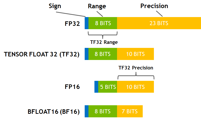
An important tradeoff is picking float16 or bfloat16, the former for more precision, the latter for more dynamic range. AMP float16 might not work with every model, and even with grad scaling to prevent underflow, this may instead cause overflow due to the numerical max of 65504 in fp16. NaNs in the loss or gradients may indicate model might not be compatible with fp16. The benefit of BF16 is that it has the same dynamic range as FP32 (same number of exponent bits).
With Ampere it also worth considering that TF32 Tensor Cores (if not already on by default) can be used with the same dynamic range as float32 except with slightly less precision (10 instead of 23 mantissa bits) - it provides essentially a free speedup.
Important: Check if TF32 is being used in runtime using torch.backends.cuda.matmul.allow_tf32 (for matmul) and torch.backends.cudnn.allow_tf32 for (cuDNN convolutions). When I checked with my PyTorch version (2.3.0) the matmul TF32 was disabled by default. In my CVAE training loop simply enabling TF32 for matrix multiplies resulted in a 1.20x speedup for backpropagation!
Set to TF32 on Ampere:
torch.backends.cuda.matmul.allow_tf32 = True
torch.backends.cudnn.allow_tf32 = True